24. Assigning probabilities (III): Conjugate priors#
In this chapter we will again use Bayes’ theorem to infer a (posterior) probability density function for parameters of the linear model, conditional on \(\data\). A large fraction of the text in this chapter was written by Andreas Ekström.
In contrast to the previous chapter on Bayesian Linear Regression (which you should have studied before reading this chapter) we will now be uncertain about the value of the variance of random errors (for simplicity we will only consider independent and identically distributed errors characterized by a single, but unknown, variance). Therefore, we are seeking to infer a joint probability density function that describes both the variance \(\sigma^2\) and the model parameters \(\pars\). Using Bayes’ theorem we can write
We will be using a normal likelihood, as written in Eq. (20.8).
The prior \(\pdf{\pars,\sigma^2}{I}\) becomes more complicated since it must describe the prior distribution of both the variance and the model parameters. Still, we want to be able to do the calculations analytically. It turns out that priors with certain functional forms facilitate analytical derivation of the posterior. These have a clever functional relationship with the relevant likelihood and are referred to as conjugate priors
24.1. A conjugate prior#
Let us define a prior probability for the model parameters \(\pars\) and \(\sigma^2\). We should of course place a prior in accordance with our prior belief about the model parameters, and our interpretation of probability. At the moment, however, we will let the mathematical structure of the likelihood guide us to choose a prior that yields an analytically tractable posterior that belongs to the same family of distributions as the prior.
Before the general availability of computers, most applied Bayesian inference focused on deriving pairs of likelihood functions and prior distributions with mathematical properties such that the posterior was analytically tractable. With the increased availability of computers, Bayesian posteriors can now be sampled numerically. Still, as you will learn in the later parts of this course, there are intrinsic challenges to sampling complex posteriors residing in high-dimensional spaces.
There are primarily three reasons for operating with a conjugate prior. First, it might actually be in accordance with our prior belief. Second, it provides insight into how the likelihood function modulates the prior to yield the posterior. Third, having closed form expressions can help us debug and verify the computational code used for sampling.
In general, a conjugate prior is constructed by factorizing the likelihood function into two parts. Somewhat simplified, one seeks a part that is independent of the parameters and another part that is dependent on the parameters. The conjugate prior is defined to be proportional to this second part. One can then show that the posterior distribution belongs to the same family as the conjugate prior. We will not show this here. Instead we will proceed with a very useful example that also enables a Bayesian interpretation of the standard linear regression method in the chapter on Linear models.
It turns out that the conjugate prior to a normally distributed likelihood, with unknown variance, is a normal-inverse-gamma prior, i.e.,
i.e., the product of the multivariate normal distribution
and the inverse-gamma distribution
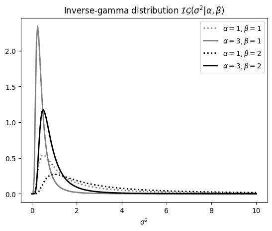
The normal distribution is well-known to you, but the inverse-gamma is perhaps a bit less familiar. It is a two-parameter distribution defined for positive real numbers, such as a variance \(\sigma^2\). The shape-parameter \(\alpha_0> 0\) governs the height of the distribution. A larger \(\alpha_0\)-value also implies thinner tails. The scale-parameter \(\beta_0>0\) governs the width of the distribution. For \(X\sim\mathcal{IG}(\alpha_0,\beta_0)\) we have
In the Python script below we plot a few instance of the \(\mathcal{IG}\) distribution. You should play with this code and convince yourself that the mean and mode of the distribution follows the expressions above.
import numpy as np
import matplotlib.pyplot as plt
from scipy.stats import invgamma

def ig_distribution(alpha,beta):
    return invgamma(a=alpha,scale=beta)

sigma2 = np.linspace(0,10,200)

hyperpars = [(1,1),(3,1),(1,2),(3,2)]
colors = ['grey','grey','black','black',]
linestyles = [':','-',':','-']

fig,ax = plt.subplots(1,1)

for ((_alpha,_beta),_color,_ls) in zip(hyperpars,colors,linestyles):
	IG = ig_distribution(alpha=_alpha,beta=_beta)
	ax.plot(sigma2,IG.pdf(sigma2),lw=2,color=_color,ls=_ls,\
		label=f'$\\alpha={_alpha},\\beta={_beta}$');

ax.set_title(r'Inverse-gamma distribution $\mathcal{IG}(\sigma^2|\alpha,\beta)$')
ax.set_xlabel(r'$\sigma^2$');
ax.legend();
Summarizing, the conjugate prior we will operate with in the following is given by
This prior depends on four parameters: \(\boldsymbol \mu_0,\boldsymbol \Sigma_0,\alpha_0,\beta_0\), where the first two define the mean (vector) and covariance (matrix) of the prior multivariate normal, and the latter two define the so-called shape (\(\alpha_0\)) and scale (\(\beta_0\)) of the inverse-gamma prior. The parameters of the prior are sometimes referred to as hyperparameters. In all our examples we will assume these to have definite values. Being Bayesian, one could place a (hyper)prior on them, but we will stop the chain of priors here.
24.2. The posterior#
At first sight, the \(\mathcal{NIG}\) prior appears clumsy but its exponential structure fits like a glove with the form of the normal likelihood and enables a closed-form expression for the resulting posterior. Combining the \(\mathcal{NIG}\) prior for \(\pars\) and \(\sigma^2\) with the normal likelihood in Eq. (20.8) one can show (see Deriving the posterior* (extra material)) that the posterior is given by
with
In effect, the prior parameters \((\boldsymbol{\mu}_0,\boldsymbol{\Sigma}_0,\alpha_0,\beta_0)\) learn from the data, and the updated posterior parameters are given by \((\widetilde{\boldsymbol{\mu}},\widetilde{\boldsymbol{\Sigma}},\widetilde{\alpha},\widetilde{\beta})\). One can also show (see Deriving the posterior* (extra material)) that the marginal posterior distributions are given by
The \(\mathcal{T}\)-distribution for a random variable \(\mathbf{Y}\in \mathbb{R}^k\) is given by
This is basically a normal distribution but with a higher probability density residing in the tails. The latter is sometimes referred to as ‘heavier tails’. They arise from the marginalization of the unknown variance of the underlying normal distribution. However, in the limit \(\nu \rightarrow \infty\) we find \(\mathcal{T}_{\nu}(\boldsymbol{\mu},\boldsymbol{\Sigma}) \rightarrow \mathcal{N}(\boldsymbol{\mu},\boldsymbol{\Sigma})\). We show in Numerical integration of the posterior (extra material) how to perform the integrals in Eq. (24.8) numerically.
Next, we will explore a useful transformation property of \(\mathcal{T}-\)distributions. Let \(\mathbf{Y}\) be a multivariate \(\mathcal{T}\)-distributed random variable. Consider a matrix \(\boldsymbol{A}\) and (column) vector \(\boldsymbol{b}\). Then, the random variable \(\mathbf{Z} = \boldsymbol{A} \mathbf{Y} + \boldsymbol{b}\) is also multivariate \(\mathcal{T}\)-distributed with the density function
The same type of identity holds for multivariate normal distributions. From this we can obtain marginal \(\mathcal{T}\)-distributions, i.e., the distributions for which we have integrated over some \(\pars\)-directions. Assume we have a \(D_1+D_2\)-dimensional \(\mathcal{T}\)-distributed random variable \(\mathbf{X} = [\mathbf{X}_1, \mathbf{X}_2]^T\), here partitioned into respective dimensions \(D_1\) and \(D_2\), with \(\boldsymbol{\mu} = [\boldsymbol{\mu}_1,\boldsymbol{\mu}_2]^T\) and
We can transform to either marginal distribution by setting, e.g.,
This yields the marginal density
Recovering the Ordinary Least Squares (OLS) result#
In our first application of the posterior in Eq. (24.6) we will reconnect with the ordinary least squares (OLS) analysis in the chapter on Linear models. This way we also build up some intuition for the general \(\mathcal{NIG}\) posterior.
It turns out that one obtain the OLS result if we tune the \(\mathcal{NIG}\) prior by setting \(\boldsymbol{\mu}_0 = 0\), \(\alpha_0 \rightarrow -N_p/2\), \(\beta_0\rightarrow 0\), and let \(\boldsymbol{\Sigma}_0\rightarrow \infty \mathbf{1}\). This particular choice of prior parameters leads to a very weakly informed prior, in fact we reach the so-called non-informative limit of the \(\mathcal{NIG}\) prior.
To understand this better, we have placed the parameter prior mean at zero and set the prior covariance matrix to a diagonal form with infinite variance. Furthermore, one can show that the limits of \(\alpha_0\) and \(\beta_0\) lead to a so-called Jeffrey’s prior for the variance: \(\p{\sigma^2} \propto 1/\sigma^2\). Some refer to Jeffrey’s priors as objective since they are invariant under coordinate transformations. We will not delve into this topic further. We will merely validate that it returns the OLS result, for which we have not specifically declared priors, only the likelihood. For the above choice of \(\mathcal{NIG}\) prior we obtain the posterior
Clearly, the parameter posterior mean \(\widetilde{\boldsymbol{\mu}}\) coincides with the OLS point estimate \(\pars^{\star}\). Furthermore, one can show that \(\widetilde{\beta}\) is proportional to the OLS sample variance \(s^2\)
We can therefor extract the OLS data variance as \(s^2=\widetilde{\beta}/\widetilde{\alpha}\). As such, we recover the OLS result as a subset of the Bayesian approach to linear regression. The upshot of the Bayesian approach is of course that it allows us to straightforwardly incorporate any prior knowledge we have, and depart the (posited) objective stance.
24.3. The posterior predictive#
Following the reasoning in the section on Deriving the posterior* (extra material) one can also derive the posterior predictive distribution (PPD), i.e., the probability distribution for predictions \(\widetilde{\boldsymbol{\mathcal{F}}}\) given the model \(M\) and a set of new inputs for the independent variable \(\boldsymbol{x}\). The new inputs also give rise to a new design matrix \(\widetilde{\dmat}\).
We obtain the posterior predictive distribution by marginalizing over the uncertain model parameters that we just inferred and that we now know follow a \(\mathcal{NIG}\) distribution
The scale of the \(\mathcal{T}\)-distribution contains two terms; the first one is \((\widetilde{\beta}/\widetilde{\alpha})\mathbf{1}\) and is directly proportional to the sample variance, and the second term \((\widetilde{\beta}/\widetilde{\alpha}) \widetilde{\dmat}\widetilde{\boldsymbol{\Sigma}}\widetilde{\dmat}^T\) is directly proportional to the covariances of the model parameters that we learned from the data
24.4. Bayesian linear regression: warmup#
To warm up, we consider the same situation as in Ordinary linear regression: warmup.
For the time being we assume to know enough about the data to consider a normal likelihood suitable. This time we also have prior knowledge that we would like to build into the inference. In a realistic situation this knowledge might come from several years of detailed studies, so called domain knowledge, consistent with a \(\mathcal{NIG}\) conjugate prior
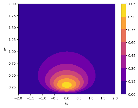
which is to say that before looking at the data we believe \(\pars\) to be centered on zero with a variance of one, and the unknown variance of the data to follow an \(\mathcal{IG}-\)distribution with mean one and mode 1/3.
Let us plot the \((\theta_i,\sigma^2)\)-marginals of this prior. The prior is the same for \(\theta_0\) and \(\theta_1\), so it is enough to plot one of them. To do so we first define a python function for the \(\mathcal{NIG}\)-distribution. You also need the inverse-gamma distribution from the Python code above.
from scipy.stats import t, norm

def normal_distribution(mu,sigma2):
    return norm(loc=mu,scale=np.sqrt(sigma2))

def t_distribution(nu,mu,sigma_hat2):
    return t(df=nu,loc=mu,scale=np.sqrt(sigma_hat2))

def nig_distribution(th,s2,mu0,Sigma0,alpha,beta):

    if alpha<=0:
        print('error alpha<=0')
        return 0
    if beta<=0:
        print('error beta<=0')
        return 0

    nig = norm.pdf(th,loc=mu0,scale=np.sqrt(s2)*np.sqrt(Sigma0))*invgamma.pdf(s2,a=alpha,scale=beta)
    return nig
Then we use python to draw a contour plot across a meshgrid. We choose the axis limits to enable easy comparison with the marginal posteriors plotted later.
x = np.linspace(-2,2,100)
y = np.linspace(0.1,2,100)

X,Y = np.meshgrid(x,y)
plt.contourf(X,Y,nig_distribution(X,Y,mu0=0,Sigma0=1,alpha=2,beta=1),cmap=plt.cm.plasma);
plt.colorbar();
plt.xlabel(r'$\theta_i$');
plt.ylabel(r'$\sigma^2$');
It is straightforward to evaluate Eq. (24.7), which gives us
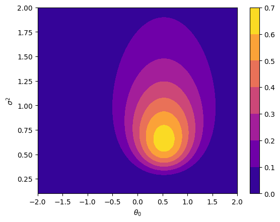
This should be compared with the parameter vector \([1,2]\) we recovered using ordinary linear regression. With Bayesian linear regression we start from an informative prior with both parameters centered on zero with unity variance and a rather wide distribution of possible \(\sigma^2\). With an increasing amount of data you will however find an increasingly narrow posterior centered on the true values of the data-generating mechanism.
We can plot the posterior \((\theta_i,\sigma^2)\)-marginals (for \(i=0,1\)) as well.
x = np.linspace(-2,2,100)
y = np.linspace(0.1,2,100)

X,Y = np.meshgrid(x,y)
plt.contourf(X,Y,nig_distribution(X,Y,mu0=0.53,Sigma0=0.35,alpha=3,beta=2.9),cmap=plt.cm.plasma);
plt.colorbar();
plt.xlabel(r'$\theta_0$');
plt.ylabel(r'$\sigma^2$');

fig2 = plt.figure();

x = np.linspace(-2,2,100)
y = np.linspace(0.1,2,100)

X,Y = np.meshgrid(x,y)
plt.contourf(X,Y,nig_distribution(X,Y,mu0=1.59,Sigma0=0.18,alpha=3,beta=2.9),cmap=plt.cm.plasma);
plt.colorbar();
plt.xlabel(r'$\theta_1$');
plt.ylabel(r'$\sigma^2$');
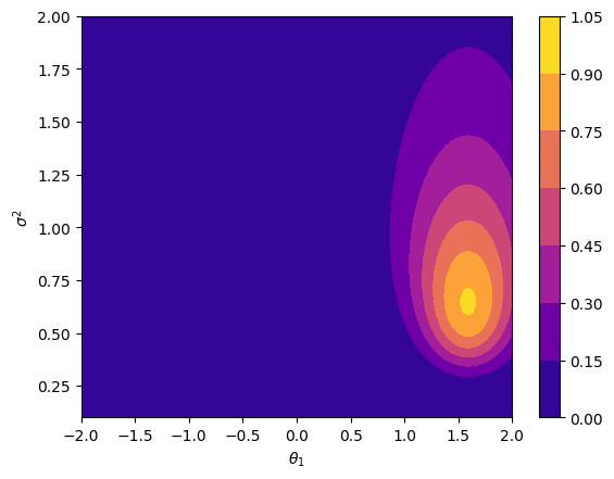
To facilitate these calculations, and easily test other priors, you can utilize Python to write a function as the one below. It takes the data vector \(\data\) and design matrix \(\dmat\) as arguments in addition to the \(\mathcal{NIG}\) prior parameters. This function is compatible with the Python functions in the chapter on Linear models. If you set the argument ‘noninformative = True’, you will obtain the OLS result (including an ill-defined sample variance).
#computes the posterior NIG parameters from data
def posterior_nig_prior(D_, X_, mu0, Sigma0, a0, b0, noninformative = False):
    # data matrix
    D = D_['data'].to_numpy()
    Nd = len(D)
    # design matrix
    X = X_.to_numpy()
    Np = len(X[0])

    #option B: non-informative prior
    if noninformative is True:
        mu0 = np.ones(Np)*0
        Sigma0_inv = np.diag(np.square(np.ones(Np)*0.0))
        a0 = -Np/2
        b0 = 0

    else:
        Sigma0_inv = np.linalg.inv(Sigma0)

    #posterior
    Sigma_inv = Sigma0_inv + np.matmul(X.T,X)
    Sigma = np.linalg.inv(Sigma_inv)
    mu = np.matmul(Sigma,np.matmul(Sigma0_inv,mu0) + np.matmul(X.T,D))

    a = a0 + Nd/2

    mSm = np.matmul(np.matmul(mu0.T,Sigma0_inv),mu0)
    DtD = np.matmul(D.T,D)
    pSp = np.matmul(np.matmul(mu.T,Sigma_inv),mu)
    b = b0 + 0.5*(mSm + DtD - pSp)

    #posterior (tilde) parameters
    return mu, Sigma, a, b
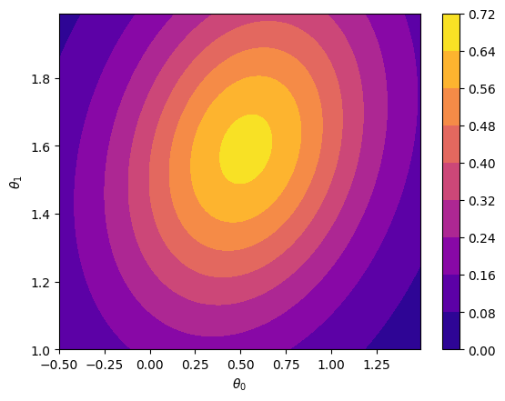
Let us also look at the marginal probability distribution (Eq. (24.8)) for \(\pars\), i.e., by plotting the bi-variate \(\mathcal{T}-\)distribution with the parameter in Eq. (24.14). We can use the Python module Scipy to evaluate many of the most common probability density functions.
from scipy.stats import multivariate_t

mu = np.array([0.53,1.59])
Sigma = np.array([[0.36,0.06],[0.06,0.18]])
a = 3
b=2.9

rv = multivariate_t(mu, (b/a)*Sigma, df=2*a)

x, y = np.mgrid[-0.5:1.5:.01, 1:2:.01]
pos = np.dstack((x, y))
plt.xlabel(r'$\theta_0$')
plt.ylabel(r'$\theta_1$')
im = plt.contourf(x, y, rv.pdf(pos),cmap=plt.cm.plasma);
plt.colorbar(im);
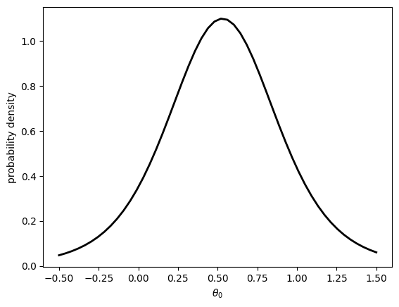
Using Eq. (24.10) we can obtain, e.g., the \(\theta_0\) marginal density
from scipy.stats import t

x = np.linspace(-0.5,1.5,50)
uv_mu = mu[0]
uv_Sigma = (b/a)*Sigma[0,0]

rv = t(df=2*a, loc=uv_mu, scale=uv_Sigma)
plt.xlabel(r'$\theta_0$')
plt.ylabel('probability density')
plt.plot(x, rv.pdf(x), 'k-', lw=2,);
The key take-away with this numerical exercise is that Bayesian inference yields a probability distribution for the model parameters whose values we are uncertain about. With ordinary linear regression techniques you only obtain the parameter values that optimize some cost function, and not a probability distribution. Using conjugate priors we can do everything analytically.
24.5. Bayesian linear regression in practice#
Next we will consider a slightly more realistic situation, although the data is still generated by us which also means that we have full knowledge of the data-generating process. In a real scenario, we have gathered some noisy data, and we try to make sense of it via some model. The goal is to infer the posterior density for the model parameters and, e.g., use this to predict data. All steps can be reproduced using the Python code provided in the code cells. You are strongly encouraged to reproduce all results yourself, and then modify the number of data points, the prior, and the underlying model. It is always instructive to explore the extremes.
Collecting the data#
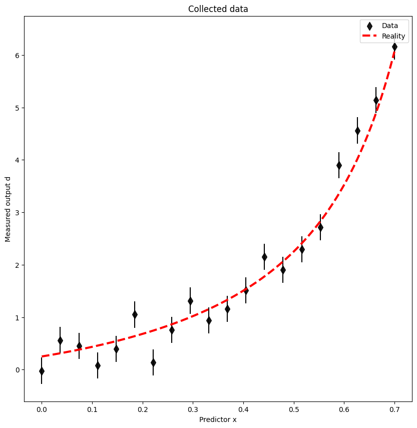
We will generate data from a function
and add a normally distributed measurement error \(\varepsilon_i \sim \mathcal{N}(0,\sigma_e^2)\) with \(\sigma_e = 0.25\). Note that all errors originate from the same normal distribution. This might not always be the case, and with unequal variances one should resort to weighted regression, which we do not cover here.
Lets assume that we perform \(N_d=20\) measurements for random \(x_i \in [0.0,0.7]\) with \(i=1\ldots 20\).
Show code cell source
import numpy as np
import pandas as pd
import matplotlib.pyplot as plt

np.random.seed(123)

def data_generating_process(model_type, seed, **kwargs):
    np.random.seed(seed)
    if model_type == 'polynomial':
        true_params = np.random.uniform(low=-5.0, high=5, size=(kwargs['poldeg']+1,))
        #polynomial model
        def process(params, xdata):
            ydata = np.polynomial.polynomial.polyval(xdata,params)
            return ydata

    elif model_type == 'nonlinear':
        true_params = None
        def process(params, xdata):
            ydata = (0.5 + np.tan(np.pi*xdata/2))**2
            return ydata

    else:
        print(f'Unknown Model')
    # return function for the true process
    #        the values for the true parameters
    #        and the name of the model_type
    return process, true_params, model_type

def measurement(data_generating_process, params, xdata, sigma_error=0.5, sigma_noise=0.0):

   ydata = data_generating_process(params, xdata)

   #  sigma_error: measurement error.
   error = np.random.normal(0,sigma_error,len(xdata)).reshape(-1,1)
   #  sigma_noise: we will also leave an option to perturb the data with some mechanism that
   #  is completely unknown to us. This will be switched off by default.
   ydata += np.random.normal(0,sigma_noise,len(xdata)).reshape(-1,1)

   return ydata+error, sigma_error*np.ones(len(xdata)).reshape(-1,)

#the number of data points to collect
Nd = 20

# predictor values
xmin = 0 ; xmax = +0.7
Xmeasurement = np.linspace(xmin,xmax,Nd).reshape(-1,1)
# store it in a Panda dataframe
pd_Xmeasurement = pd.DataFrame(Xmeasurement, columns=['x'])

# Define the data-generating process.
# Begin with a polynomial (poldeg=1) model_type
# in a second run of this notebook you can play with other linear models
reality, true_params, model_type = data_generating_process(model_type='nonlinear',seed=123, poldeg=3)

print(f'model type: {model_type}')
print(f'true parameters: {true_params}')

print(f'Nd = {Nd}')

# generate a denser grid to evaluate the linear model. This is useful for plotting

xdense = np.linspace(xmin,xmax,200).reshape(-1,1)
pd_R = pd.DataFrame(reality(true_params,xdense), columns=['data'])
pd_R['x'] = xdense

# Collect the data
sigma_e = 0.25
Ydata, Yerror = measurement(reality,true_params,Xmeasurement, sigma_error = sigma_e)
# store the data in Panda dataframes
pd_D=pd.DataFrame(Ydata,columns=['data'])
#
pd_D['x'] = Xmeasurement
pd_D['e'] = Yerror

# helper function to plot data, reality, and model (pd_M)
def plot_data(pd_D, pd_R, pd_M, with_errorbars = True):
    fig = plt.figure(figsize=(10,10))
    plt.scatter(pd_D['x'],pd_D['data'],label=r'Data',color='black',zorder=1, alpha=0.9,s=70,marker="d");
    if with_errorbars:
        plt.errorbar(pd_D['x'],pd_D['data'], pd_D['e'],fmt='o', ms=0, color='black');
    if pd_R is not None:
        plt.plot(pd_R['x'], pd_R['data'],color='red',linestyle='--',lw=3,label='Reality',zorder=10)
    if pd_M is not None:
        plt.plot(pd_M['x'], pd_M['data'],color='blue',linestyle='--',lw=3,label='Model',zorder=11)
    plt.ylabel('output');
    plt.legend();
    plt.title('Collected data');
    plt.xlabel(f'Predictor x');
    plt.ylabel(f'Measured output d');
model type: nonlinear
true parameters: None
Nd = 20
Here we plot the data as well as the data-generating process (‘reality’, red dashed line). This is a monotonically increasing function across the interval in the figure.
plot_data(pd_D, pd_R, None)
Setting up a linear model#
The data is generated by a nonlinear process, but we will pretend to not know this. Instead we will try to interpret this data using a theory that is grounded in the method of Taylor expansion. In fact, this is quite common in physics although the expansion might be of different origin. This is also a good example of a situation where the model is wrong, and in a more advanced analysis we would try to incorporate a model for this discrepancy (see Data, models, and predictions) using our knowledge about the remainder term of Taylor expansions.
Nevertheless, we will now analyze the data using a linear model with polynomial basis functions up to order \(N_p-1\), where \(N_p\) is the number of unknown parameters \(\pars\) multiplying the basis functions (See Eq.(7.2)). We will start with a 6th order polynomial, i.e., \(N_p=7\). In the exercises below you will explore other options.
Show code cell source
def setup_polynomial_design_matrix(data_frame, poldeg, drop_constant=False, verbose=True):
    if verbose:
        print('setting up design matrix:')
        print('  len(data):', len(data_frame.index))

        # for polynomial models: x^0, x^1, x^2, ..., x^p
        # use numpy increasing vandermonde matrix
        print('  model poldeg:',poldeg)

    predictors = np.vander(data_frame['x'].to_numpy(), poldeg+1, increasing = True)
    if drop_constant:
        predictors = np.delete(predictors, 0, 1)
        if verbose:
            print('  dropping constant term')
    pd_design_matrix = pd.DataFrame(predictors)

    return pd_design_matrix

Np = 7
pd_X = setup_polynomial_design_matrix(pd_Xmeasurement,poldeg=Np-1)
pd_Xreality = setup_polynomial_design_matrix(pd_R,poldeg=Np-1)
setting up design matrix:
  len(data): 20
  model poldeg: 6
setting up design matrix:
  len(data): 200
  model poldeg: 6
Taylor expanding Eq. (24.15) tells us that values of the model parameters \(\pars\) should be in the vicinity of
Inference using a non-informative prior#
In a first attempt, we use Bayesian linear regression with a non-informative \(\mathcal{NIG}\) prior by calling the relevant Python function defined above. Using a non-informative prior of this kind will of course yield a result identical to the one obtained using ordinary linear regression.
mu0 = None
Sigma0 = None
a0 = None
b0 = None
mu, Sigma, a, b = posterior_nig_prior(pd_D, pd_X, mu0, Sigma0, a0, b0, noninformative=True)

print(f'Mean values of parameters theta_i:')
for idx, this_mu in enumerate(mu):
    print(f'theta {idx}: {this_mu:.3f}')

print(f'\n Estimate of data variance s^2: {(b/a):.3f}')

#store the results in a Panda dataframe
Xreality = pd_Xreality.to_numpy()
pd_M_bayes = pd.DataFrame(np.matmul(Xreality,mu),columns=['data'])
pd_M_bayes['x'] = xdense
Mean values of parameters theta_i:
theta 0: 0.048
theta 1: 15.117
theta 2: -209.025
theta 3: 1249.294
theta 4: -3400.193
theta 5: 4335.647
theta 6: -2064.814

 Estimate of data variance s^2: 0.098
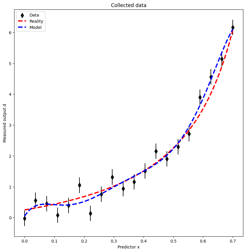
Note that the parameters \(\theta_i\) attain alternating positive and negative values, for the most part, and that the numerical values are quite large. Plotting the result also tells us that we are most likely overfitting the parameters at low values for \(x\), i.e., we are picking up noise from the data. This is often a consequence in situations where we have too little data to justify a large number of parameters, seven in this case.
plot_data(pd_D, pd_R, pd_M_bayes)
Inference using an informative prior#
Next we will try to tame the regression such that the inferred values for the parameters \(\pars\) reside in the vicinity of one. There might be several reasons for this. Extrapolation using a polynomial with wildly varying parameter values will most likely not work well. Using machine learning jargon, we might say that the trained model will not generalize beyond the training data. From a physics point of view, it is often reasonable to assume that the parameter values, when rescaled to dimensionless units, should be of order one. This is consistent with a so-called naturalness hypothesis. There might be other reasons for why one seeks \(\pars \approx \mathcal{O}(1)\). In the Bayesian approach we can inject such assumptions using the prior. In this example, we place the following prior
where we also assumed some uncertainty in our prior for the parameter values. Based on the magnitudes of the error bars we also set
With this prior, and a normal likelihood for the data, we obtain the following posterior density for the model parameters
mu0    = np.ones(Np)
Sigma0 = 100*np.eye(Np)
a0 = 2
b0 = 2
mu, Sigma, a, b = posterior_nig_prior(pd_D, pd_X, mu0, Sigma0, a0, b0, noninformative=False)

print(f'Mean values of parameters theta_i:')
for idx, this_mu in enumerate(mu):
    print(f'theta {idx}: {this_mu:.3f}')

print(f'\n Estimate of data variance s^2: {(b/a):.3f}')

#store the results in a Panda dataframe
Xreality = pd_Xreality.to_numpy()
pd_M_bayes = pd.DataFrame(np.matmul(Xreality,mu),columns=['data'])
pd_M_bayes['x'] = xdense
Mean values of parameters theta_i:
theta 0: 0.228
theta 1: 0.748
theta 2: 3.258
theta 3: 4.485
theta 4: 4.469
theta 5: 3.938
theta 6: 3.296

 Estimate of data variance s^2: 0.249
Plotting the Bayesian linear model, using an informative prior, together with the data and the data-generating process looks like this:
plot_data(pd_D, pd_R, pd_M_bayes)
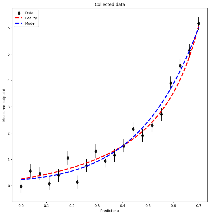
Clearly, with the informative prior above we have successfully managed to infer a model with more reasonable values for the model parameters. The full posterior \(\pdf{\pars,\sigma^2}{\data}\) is an 8-dimensional \(\mathcal{NIG}\) density with 7 parameters \([\theta_0,\theta_1,\ldots,\theta_6]\) and the inferred variance \(\sigma^2\). To easily visualize this distribution we will can plot (at most) two parameter combinations at the time. When arranging all plots on a grid, with the univariate marginal distributions on the diagonal, the result is often referred to as a corner plot.
To obtain marginal posteriors in our case, we can use Eq. (24.10), as was done in Bayesian linear regression: warmup. An alternative to this is numerical sampling of the analytical posteriors. Indeed, using the scipy Python library we have access to most of probability distributions and methods for drawing random samples distributed accordingly. Although, the \(\mathcal{NIG}\) density is not part of the standard set in scipy. Instead, we draw one \(\sigma^2 \sim \mathcal {IG}(\alpha,\beta)\) and subsequently draw one \(\pars \sim \mathcal{N}(\boldsymbol{\mu},\sigma^2 \boldsymbol{\Sigma})\). Then we repeat this \(n_{\rm samples}\) times. See the python code below.
To draw the corner plot we utilize the library prettyplease.
# Pretty corner plots generated with `prettyplease`
# https://github.com/svisak/prettyplease
import sys
import os
from scipy.stats import multivariate_normal

# Adding ../Utils/ to the python module search path
sys.path.insert(0, os.path.abspath('../../Utils/'))

import prettyplease.prettyplease as pp

IG_posterior = invgamma(a,b)

n_samples = 10000
n_dim = Np

NIG_samples = []
for i in range(n_samples):
    sig2 = IG_posterior.rvs(1)
    mvn = multivariate_normal(mu,sig2*Sigma)
    theta = mvn.rvs(1)
    sample = np.concatenate((theta,sig2))
    NIG_samples.append(sample)

x = np.array(NIG_samples)
labels = [rf'$\theta_{i}$' for i in range(n_dim)] + [rf'$\sigma^2$']
fig = pp.corner(x,bins=30, labels=labels,colors='blue',title_loc='center',n_uncertainty_digits=2,figsize=(14,14))
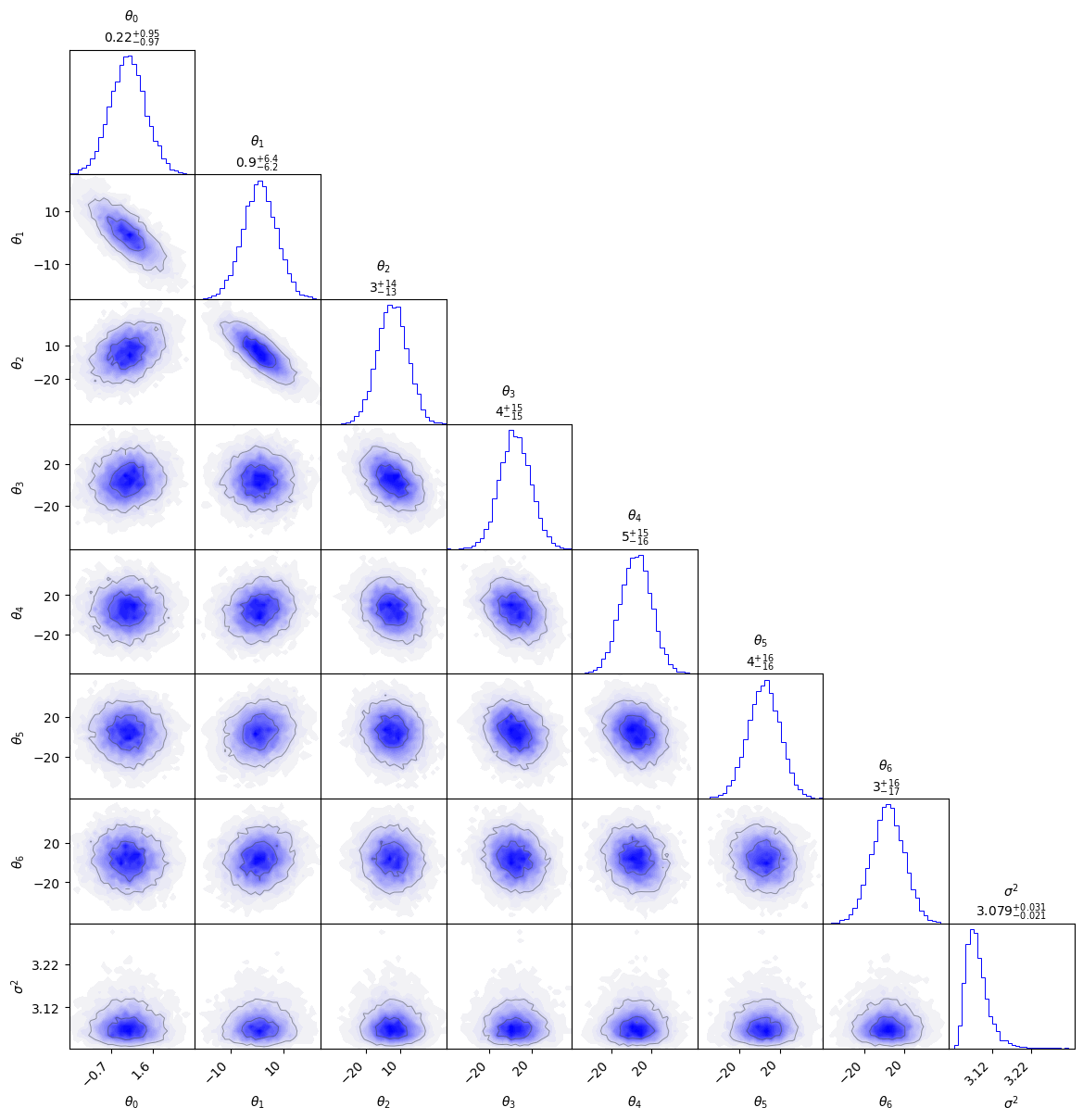
The procedure of taming the model parameters during inference is also called regularization. The goal (hope) of doing so is to make the model generalize better and thereby increase the predictive accuracy. This is a common technique employed to prevent overfitting and used extensively in machine learning. From a Bayesian perspective, regularization is often (mathematically) equivalent amounts to imposing a certain prior distribution on the model parameters. This is discussed briefly in the extra material on Regularization* (extra material).
In the exercises below you are encouraged to explore different models and their predictions based on non-informative and informative priors. One should always keep in mind that there is no silver bullet to obtain accurate predictions. Make accurate predictions requires reliable information and an accurate model.
Quantifying the posterior predictive distribution#
We will end this section on Bayesian linear regression with an example on how to quantify the The posterior predictive in practice. The model parameters are represented as posterior probability distributions \(\pdf{\pars,\sigma^2}{\data}\), and equation (24.13) tells us that we must average any model prediction with respect to this posterior, and when operating with a linear model and conjugate prior the resulting posterior predictive is analytically tractable.
First, we define the vector of values for the independent variable \(\mathbf{x}\) that we wish to make predictions for. In this case we would like to obtain a somewhat smooth representation, and the model is very fast to evaluate, so we opt for 200 values for \(x \in [0.0,0.8]\). This interval encompasses the range for which we have historic data employed during the model inference, i.e., \([0.0,0.7]\). Next, we construct the design matrix of model predictions \(\widetilde{\dmat}\)
xmax_f = +0.8
xdense_new = np.linspace(xmin,xmax_f,200).reshape(-1,1)
pd_xnew = pd.DataFrame(xdense_new, columns=['x'])
pd_XF = setup_polynomial_design_matrix(pd_xnew,poldeg=Np-1)
setting up design matrix:
  len(data): 200
  model poldeg: 6
Knowing the parameter values that characterize the posterior (\(\boldsymbol{\mu},\boldsymbol{\Sigma},\alpha,\beta\)), we can easily evaluate the posterior predictive density at all values of the independent variable \(\mathbf{x}\). In the following we will extract the 95% credible interval of the posterior predictive, and we choose the highest density region (see Point estimates and credible regions). The result is indicated with a filled blue region, and the mean value as a dark blue line. The python code below loops over all rows of the design matrix and stores the mean and 95% credible interval for each value of the independent variable.
XF = pd_XF.to_numpy()

ci_level = 0.95 # set the level of the credible interval

mean = []
ci_lo = []
ci_hi = []
for row in XF:
    Xmu = row@mu
    scale = (b/a)*(1+row@Sigma@row.T)
    t_ppd = t(2*a,Xmu,scale)
    mean.append(t_ppd.mean())
    lo, hi = t_ppd.interval(ci_level)
    ci_lo.append(lo)
    ci_hi.append(hi)


#the number of data points predictions between [xmax, and xmax_f] (defined in the cell above)
Nd_f = 10

# predictor values
Xmeasurement_f = np.linspace(xmax,xmax_f,Nd_f).reshape(-1,1)
# store it in a Panda dataframe
pd_Xmeasurement_F = pd.DataFrame(Xmeasurement_f, columns=['x'])

# Collect the predicted data
Ydata_f, Yerror_f = measurement(reality,true_params,Xmeasurement_f, sigma_error = sigma_e)
# store the data in Panda dataframes
pd_DF=pd.DataFrame(Ydata_f,columns=['data'])
# store the new data
pd_DF['x'] = Xmeasurement_f
pd_DF['e'] = Yerror_f

# plot everything!
fig = plt.figure(figsize=(10,10))
plt.plot(xdense_new,mean,color='blue',lw=3,label=f'Mean');
plt.plot(xdense_new,ci_hi,color='blue',ls=':',lw=1.5);
plt.plot(xdense_new,ci_lo,color='blue',ls=':',lw=1.5);

xx = np.array(xdense_new).reshape(-1);
lo = np.array(ci_lo).reshape(-1);
hi = np.array(ci_hi).reshape(-1)
plt.fill_between(xx,lo,hi,alpha=0.2,label=f'{ci_level*100:.0f}% credible interval');

plt.scatter(pd_D['x'],pd_D['data'],label=r'Data',color='black',zorder=1, alpha=0.9,s=70,marker="d");
plt.errorbar(pd_D['x'],pd_D['data'], pd_D['e'],fmt='o', ms=0, color='black');

plt.scatter(pd_DF['x'],pd_DF['data'],label=r'New data',color='red',zorder=1, alpha=0.9,s=70,marker="d");
plt.errorbar(pd_DF['x'],pd_DF['data'], pd_DF['e'],fmt='o', ms=0, color='red');

plt.title('Model prediction');
plt.xlabel('Predictor x');
plt.ylabel('Measured output d');
plt.legend();
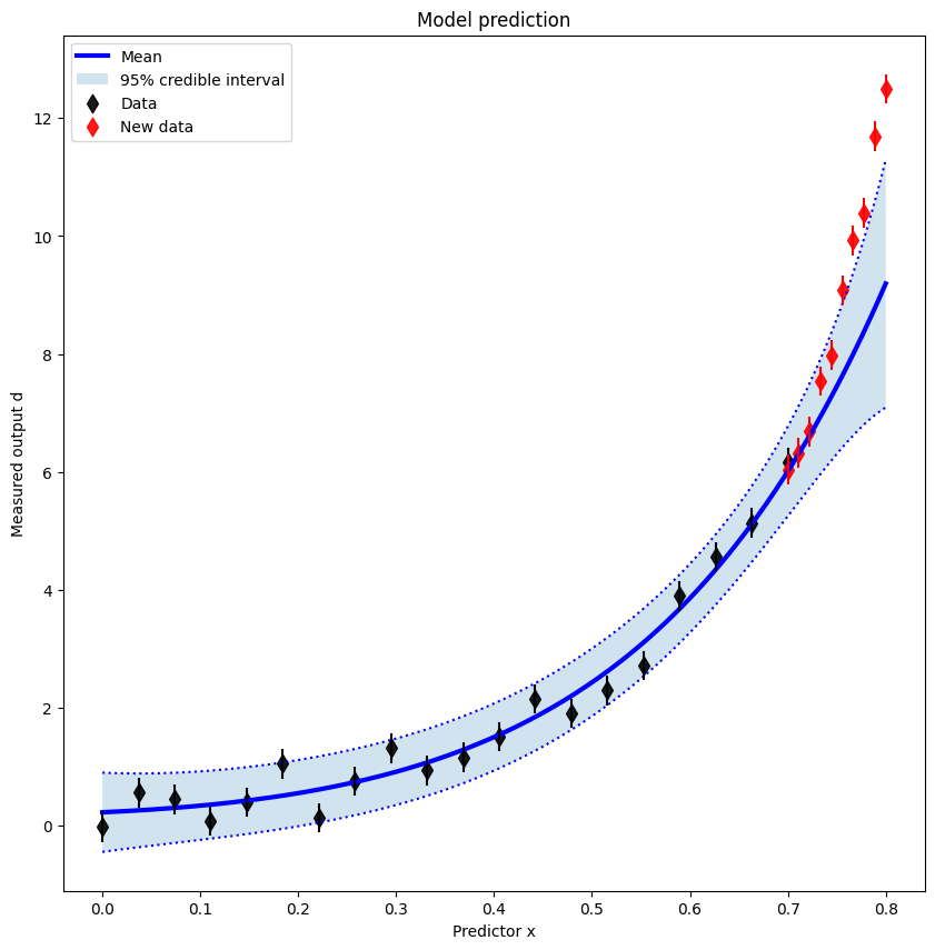
Let us discuss this result. The credible interval provides valuable insight into how certain we are of the model prediction conditional on all our assumptions and the historic data. It is obvious that all new data does not fall in this credible interval, in particular if we extrapolate further away from the region where we have historic data. This is reasonable since our model is wrong
24.6. Numerical integration of the posterior (extra material)#
extra material
Let us do the integrals in (24.8) numerically using Python. For this you can use a standard Riemann sum, or if you are acquainted with Gauss-Legendre quadrature, even better. The code below is equipped with both options. Although we should take the upper integration limit to infinity, we settle for a relatively large number. This can be improved upon by approximate numerical mapping of the finite interval \([a,b]\) to \([0,\infty]\). To facilitate evaluation of the \(\mathcal{NIG}\) integrand, we setup a function using the Python ‘lambda’ syntax.
Next we setup a function to deliver integration meshes to do quadrature,
def integration_mesh(N,a,b, gauleg=False):
    if gauleg:
        # gauss legendre integration between [a,b] using N-point quadrature
        x, w = np.polynomial.legendre.leggauss(N)
        # Translate x values from the interval [-1, 1] to [a, b]
        tt = 0.5*(x + 1)*(b - a) + a
        uu = w * 0.5*(b - a)
    else:
        # standard riemann sum of N-term across the interval [a,b]
        tt = np.linspace(a,b,N)
        uu = (b-a)/N
    return tt,uu
extra material
Define the \(\mathcal{NIG}\) parameters as well as the \(\mathcal{NIG}\) function which we will integrate and the analytical \(\mathcal{T}-\) & \(\mathcal{IG}\)-distributions to compare with
# set the values of the NIG paramters you would like to run with.
mu = 0
Sigma = 1
alpha = 1
beta = 1
nu=2*alpha

fNIG = lambda th,s2: nig_distribution(th,s2,mu,Sigma,alpha,beta)
fT  = t_distribution(nu,mu,(beta/alpha)*Sigma)
fIG = ig_distribution(alpha,beta)
extra material
Now we perform the integration and plot the numerical result (red dotted) for comparison with the respective analytical expression in Eq. (24.8) (black solid) for the two marginals.
#marginalize NIG wrt sigma^2
s2,w = integration_mesh(100,1e-16,+40)
theta = np.arange(-5,5,0.01)
NIG_marginalized_sigma2 = []
for th in theta:
    NIG_marginalized_sigma2.append(np.sum(fNIG(th,s2)*w))

#marginalize NIG wrt theta
th,w = integration_mesh(100,-30,+30)
sigma2 = np.arange(1e-6,5,0.01)
NIG_marginalized_theta = []
for s2 in sigma2:
    NIG_marginalized_theta.append(np.sum(fNIG(th,s2)*w))

plt.title(r'$\mathcal{T}_{\nu=%d}(\theta|\mu=%.1f,\hat{\sigma}^2=%.1f)$'%(nu,mu,Sigma));
plt.xlabel(r'$\theta$');
plt.plot(theta,fT.pdf(theta),label='analytical',linestyle='-',color='black',linewidth=3);
plt.plot(theta,NIG_marginalized_sigma2,label=f'numerical',linestyle=':',color='red',linewidth=6);
plt.legend();

fig2 = plt.figure();

plt.title(r'$\mathcal{IG}(\sigma^2|\alpha=%.1f,\beta=%.1f)$'%(alpha,beta));
plt.xlabel(r'$\sigma^2$');
plt.plot(sigma2,fIG.pdf(sigma2),label='analytical',linestyle='-',color='black',linewidth=3);
plt.plot(sigma2,NIG_marginalized_theta,label=f'numerical',linestyle=':',color='red',linewidth=6);
plt.legend();
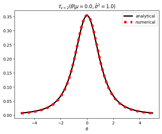
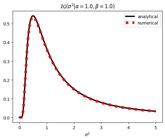
extra material
We have now shown that the posterior for the vector of (linear) model parameters follows a multivariate \(\mathcal{T}-\)distribution \(\mathcal{T}_{\nu}(\pars|\boldsymbol{\mu},\boldsymbol{\Sigma})\) which has three parameters: \(\nu\) (degrees of freedom), \(\boldsymbol{\mu}\) (median, mode, and mean if \(\nu>1\)), and \(\boldsymbol{\Sigma}\) (scale matrix).
24.7. Regularization* (extra material)#
extra material
discuss different norms in regression and priors in Bayes LinReg
24.8. Deriving the posterior* (extra material)#
extra material
This section contains extra material for to derive the expressions for the posterior parameters in Eq. (24.7) and the marginal posteriors in Eq. (24.8). One strategy for deriving this is to exploit the known properties of conjugate priors and the normalization factors. We will take a slightly longer route. To shorten some of the expressions we will sometimes operate with unconditional probabilities, and assume implicit conditioning on \(I\) in case nothing else applies.
We begin by multiplying the likelihood and the prior in Eq. (20.8) and Eq. (24.5), respectively. Applying Bayes’ theorem immediately tells us that the posterior is proportional[1] to
where we also defined a shorthand \(E\) for part of the exponent.
Expanding the products in \(E\) gives
Let us collect the terms that are linear and quadratic in \(\pars\).
One can show the following matrix identity[2] for a symmetric matrix \(\mathbf{A}\) and vectors \(\mathbf{x}\) and \(\mathbf{a}\)
If we assume that our design matrix \(\dmat\) is invertible, i.e., that there are no linearly dependent columns, then the product \(\dmat^{T}\dmat\) is a symmetric matrix[3]. Then we can apply the identity in Eq. (24.18) to our exponent term \(E\). This will allow us to rewrite \(E\) such that the structure of a normal distribution becomes apparent. This will be the first step towards identifying the \(\mathcal{NIG}\) form of the posterior in Eq. (24.17). We obtain
Now, only the first term depends on \(\pars\). Using the tilde-shorthand defined in Eq. (24.6), we can write the entire exponential factor in Eq. (24.17) as
To obtain the full posterior distribution in Eq. (24.6) we have to normalize the expression in Eq. (24.17). For this we have to compute the marginal likelihood given by
We will start with the integral over \(\pars\) and compute the likelihood function \(\pdf{\data}{\sigma^2}\). The product of two normal distributions can be re-written by completing the square, yielding an integrand consisting of a single normal distribution, with a known normalization constant. As an alternative, we will demonstrate another route. This requires the following known relation: For a normally distributed vector \(\mathbf{x} \sim \mathcal{N}(\boldsymbol{\mu}_x,\boldsymbol{\Sigma}_x)\), the linearly transformed vector \(\mathbf{y} = \mathbf{A}\mathbf{x} + \mathbf{b}\), where \(\mathbf{A} \in \mathbb{R}^{N \times N}\), is also normally distributed with \(\mathbf{y} \sim \mathcal{N}(\mathbf{A}\mu_x + \mathbf{b}, \mathbf{A}\boldsymbol{\Sigma}_x\mathbf{A}^T)\). For our linear model \(\dmat\pars + \boldsymbol{\varepsilon}\) with \(\boldsymbol{\varepsilon} \sim \mathcal{N}(0,\sigma^2\mathbf{1})\) we have independently assumed
which then implies
Thus we obtain for the marginal likelihood conditional on \(\sigma^2\)
This is a normal distribution, as expected. Multiplying this with the remaining inverse-gamma prior for \(\sigma^2\) and integrating over \(\sigma^2\) will yield the total marginal likelihood. We perform this integration next. However, we will do the slightly more agnostic integral \(\mathcal{I}\) with an unspecified covariance \(\sigma^2 \boldsymbol{\Sigma_0}\). In the following expressions we suppress the zero subscript for \(\alpha\) and \(\beta\).
To make this expression easier to read, we define the integral \(\mathcal{I}\)
with
A change of variables \(t=B/\sigma^2\) leads to
If we now restore the original variables and consolidate factors we obtain
The final distribution in the last line is a so-called (multivariate) \(t\)-distribution. If we introduce the notation \(\nu = 2\alpha\) and \(\boldsymbol{\Sigma} = (\beta/\alpha)\boldsymbol{\Sigma}_0\), we obtain the standard expression for the distribution of a \(t\)-distributed vector quantity \(\mathbf{Y}\) (with \(p\) components, i.e., we also set \(N_d = p\)),
The marginal likelihood can therefore be expressed as
We now have all the pieces of the puzzle, i.e., Eqs. (24.17), (24.19), and (24.21), to form the normalized posterior using Bayes’ theorem
To evaluate the right-hand side, we begin by re-writing the denominator to match the form of the numerator.
We can use the generalized matrix determinant lemma[4] to evaluate the determinant in the denominator of the first factor in Eq. (24.22),
where we used the definition of \(\tilde{\boldsymbol{\Sigma}}\) according to Eq. (24.6).
The exponential term of the unnormalized posterior, Eq. (24.19), is written compactly using the tilde-notation defined in Eq. (24.6). We therefore need to express the second factor of the marginal likelihood in Eq. (24.22) using the same shorthand.
In fact, one can show the following equality.
To do so requires a few intermediate steps. So let us repeat them here. We will manipulate the expression above such that the right-hand equals the left-hand side. We begin by expanding the last term on the right-hand side
To get the second equality we also used that \(\tilde{\boldsymbol{\Sigma}}^T= \tilde{\boldsymbol{\Sigma}}\). The above leads to the following expression for the entire right-hand side in Eq. (24.23).
We can use the Woodbury identity[5] twice to express the middle factor of the second term using mainly the design matrix. This will enable us to form the product \(\dmat\boldsymbol{\mu}_0\) that we find in the left-hand side of Eq. (24.23).
In the second equality we used the Woodbury identity “backwards” to deflate the sum of prior covariances, and in the third equality we used it “forwards” to inflate the expression again but this time in terms of the square of the design matrix.
We now find the common factor \((\mathbf{1} - \dmat\tilde{\boldsymbol{\Sigma}}\dmat^T)\) in all terms of Eq. (24.24) except the last one. However, we can re-write \(\dmat\tilde{\boldsymbol{\Sigma}}\boldsymbol{\Sigma}_0^{-1}\).
With this in place, we can re-write Eq. (24.24) as a familiar sum of squared residuals
We now use the Woodbury identity one last time to re-write the middle factor
and we have finally demonstrated the equality in Eq. (24.23).
Going back to the expression for the marginal likelihood in terms of the multivariate \(t\)-distribution, we therefore have
Using the definitions of \(\tilde{\alpha}\) and \(\tilde{\beta}\) according to Eq. (24.6) yields
Several factors cancel when we divide the un-normalized posterior in Eq. (24.17) with the above, and the final expression for the posterior distribution is given by the \(\mathcal{NIG}\) distribution given in Eq. (24.6):
Using Eq. (24.21) we obtain the posterior marginal for \(\pars\)
and the posterior marginal for \(\sigma^2\) follows straightforwardly from integration
24.9. Exercises#
Exercise 24.1
Derive the expressions for the mean of the \(\mathcal{IG}\) distribution in Eq. (24.4).
Exercise 24.2
Derive the expressions for the mode of the \(\mathcal{IG}\) distribution in Eq. (24.4).
Exercise 24.3
In the limit of \(\nu \rightarrow \infty\), the \(\mathcal{T}(\boldsymbol{\mu},\boldsymbol{\Sigma})\)-distribution approaches a normal distribution \(\mathcal{N}(\boldsymbol{\mu},\boldsymbol{\Sigma})\). Why?
Exercise 24.4
Demonstrate numerically using Python that in the limit of \(\nu \rightarrow \infty\), the \(\mathcal{T}(\boldsymbol{\mu},\boldsymbol{\Sigma})\)-distribution approaches a normal distribution \(\mathcal{N}(\boldsymbol{\mu},\boldsymbol{\Sigma})\).
Exercise 24.5
Use the python code in this chapter to explore the posterior predictive distribution of a Bayesian linear model with polynomial basis functions up to the 7th order and a non-informative \(\mathcal{NIG}\)-prior. How well does the model generalize outside the domain of collected data used to infer the model parameters?
Exercise 24.6
Use the python code in this chapter to explore the posterior predictive distribution of a Bayesian linear model where you employ a linear model with polynomial basis functions up to the 11th order and an informative prior. Can you explain why the posterior predictive distribution is better compared to when using a 7th order polynomial?
24.10. Solutions#
Here are answers and solutions to selected exercises.
Solution to Exercise 24.1
The mean \(\mathbb{E}[X]\) of a random variable \(X\) distributed as \(\p{x}\) is given by
Thus we must solve the integral
where the expression in brackets is the \(\mathcal{IG}\)-distribution. To solve this we must also remember that the gamma function is defined as
with the interesting property that \(\Gamma(n) = (n-1)!\) for positive integers \(n>1\). A substitution of variables \(\frac{\beta}{x} = t\) yields
for \(\alpha>1\).
Solution to Exercise 24.2
To find the mode(s) we must solve for the \(x\)-value(s) where the distribution \(\p{x}\) attains a maximum(s) (lat. maxima, of course). Differentiation of the \(\mathcal{IG}-\)distribution leads to an equation in \(x\)
which is solved by