15. Bayes’ theorem#

“Prediction is very difficult, especially about the future.”

—Niels Bohr

Here we will introduce Bayes’ theorem, which you will see is the starting point for all Bayesian methods. We will explain how it encapsulates the process of learning from data, and show how it results from foundational axioms of probability theory. Therefore, our presentation also merits some philosophical remarks on the interpretation of probabilities. Finally, we will show a first application of Bayes’ theorem with the classical example of a coin tossing experiment.

15.1. Axioms of probability theory#

Andrey Kolmogorov’s axioms of probability form the standard theoretical framework in which the probability (measure) \(\mathbb{P}\) is introduced. You encountered those axioms in the definition of The probability measure. The most important aspect of his formalization of probability is not the axioms themselves but rather that he showed that probabilities can be incorporated into mathematics using the existing theory of measures. In fact, since then other axiomatic constructs of probability where, e.g., the conditional probability is taken as the primitive notion, has been constructed. In this course we rely on Kolmogorov’s axioms from which the following two useful rules for how to manipulate probabilities and uncertainties can be derived

Property 15.1 (Product rule)

(15.1)#\[\begin{equation} \prob(A, B | I) =\prob(B|A, I) \prob(A|I) = \prob(A|B,I)\prob(B|I) \end{equation}\]

The left-hand side should be interpreted as the probability for propositions \(A\) AND \(B\) being true given that \(I\) is true. The probabilities on the right hand side(s) are conditioned differently and the second equality follows from the symmetry of the AND operation.

Property 15.2 (Sum rule)

(15.2)#\[\begin{equation} \prob(A + B | I) = \prob(A | I) + \prob(B | I) - \prob(A, B | I) \end{equation}\]

The left-hand side should be interpreted as the probability for proposition \(A\) OR \(B\) being true given that \(I\) is true. If \(A\) and \(B\) are exclusive on \(I\), i.e., cannot occur simultaneously, then the third term equals zero.

15.2. Bayes’ theorem#

From the product rule we obtain Bayes’ theorem

Property 15.3 (Bayes’ rule/theorem)

(15.3)#\[\begin{equation} \prob(A|B,I) = \frac{\prob(B|A,I)\prob(A|I)}{\prob(B | I)} \end{equation}\]

The left-hand side should be interpreted as the the probability that proposition \(A\) is true given that \(B\) AND \(I\) are true. This equation tells us how we can reverse a conditional probability. More importantly it updates the probability for \(A\) being true as we learn more about \(B\).

Although Bayes’ rule is a straightforward rewrite of the product rule, its importance cannot be understated. Indeed, since this is a rule for probabilities it is applicable in all scientific analyses that follow from Kolmogorov’s axioms and it tells us how we should learn from data or react to new evidence or how new information should change our views. It is however not a rule (or theorem) that is unique to Bayesian inference.

The importance of this theorem for data analysis becomes apparent if we replace \(A\) and \(B\) by a proposed hypothesis \(H\) and data \(\data\) such that it becomes

(15.4)#\[ \prob(H|\data,I) = \frac{\prob(\data|H,I)\prob(H|I)}{\prob(\data | I)}. \]

The power of Bayes’ theorem lies in the fact that it relates the quantity of interest, the probability that the hypothesis is true given the data, to the term we have a better chance of being able to assign, the probability that we would have observed the measured data if the hypothesis was true.

Ingredients of Bayes’ theorem

The various terms in Bayes’ theorem have formal names.

The quantity on the far right, \(\prob(H|I)\), is called the prior probability; it represents our state of knowledge (or ignorance) about the truth of the hypothesis before we have analysed the current data.
This is modified by the experimental measurements through \(\prob(\data|H,I)\), the likelihood function,
The denominator \(\prob(\data | I)\) is called the evidence. It does not depend on the hypothesis and can be regarded as a normalization constant.
Together, these yield the posterior probability, \(\prob(H|\data,I)\), representing our state of knowledge about the truth of the hypothesis in the light of the data.

In a sense, Bayes’ theorem encapsulates the process of learning.

The friends of Bayes’ theorem#

Normalization and marginalization

Given an exclusive and exhaustive list of hypotheses, \(H_i\), we must have a normalization of the total probability

(15.5)#\[\begin{equation} \sum_i \prob(H_i|I) = 1, \end{equation}\]

which also leads to the marginalization property

(15.6)#\[\begin{equation} \prob(A|I) = \sum_i p(H_i|A,I) p(A|I) = \sum_i p(A,H_i|I), \end{equation}\]

where we used the product rule in the second step.

For example,let’s imagine that there are five candidates in a presidential election; then \(H_1\) could be the proposition that the first candidate will win, and so on. The probability that \(A\) is true, for example that unemployment will be lower in a year’s time (given all relevant information \(I\), but irrespective of whoever becomes president) is given by \(\sum_i \prob(A,H_i|I)\) as shown by using normalization and applying the product rule.

The continuum limit#

In the continuum limit we will replace discrete propositions \(X_i\) by a continuous variable \(X\). Rather than discrete probabilities \(\prob(X_i|I)\), the fundamental quantity will then be the probability density function \(p_X(x|I)\) that we usually write simply as \(p(x|I)\) (see Definition 6.7).

Normalization and marginalization in the continuum limit

The normalization for a continuous, conditional PDF is

(15.7)#\[\begin{equation} \int dx p(x|I) = 1, \end{equation}\]

while the marginalization property corresponds to

(15.8)#\[\begin{equation} p(y|I) = \int dx p(x,y|I). \end{equation}\]

Marginalization is a very powerful device in data analysis because it enables us to deal with nuisance parameters; that is, quantities which necessarily enter the analysis but are of no intrinsic interest. The unwanted background signal present in many experimental measurements is an example of a nuisance parameter.

15.3. Philosophical remarks on probabilities#

The axioms of probability theory are very useful for manipulating probabilities and obtaining quantitative results. There is, however, an ongoing philosophical discussion centered on the question what is the probability \(\prob\)? There exists several interpretations of probability, and the two main views are: frequentist probability and Bayesian probability. There are numerous flavors of probability interpretations in each category, most of which are consistent with Kolmogorov’s axioms. Generally speaking, there is no difference in the calculus of Bayesian and frequentist probabilities. However, their interpretations differ on a fundamental level, and we will get to that shortly. But why even bother to dwell on this topic? Philosophy is sometimes (rightly) accused of dealing solely with abstractions separated from reality and therefore of no use to someone interested in real-world applications. There is however something fundamentally useful about the philosophy of probability in the sense that all events, propositions, and outcomes in social and natural sciences are bearers of probability. It is therefore of fundamental importance to learn how we can use the mathematical measure of probability to better understand real systems.

Frequentist probability#

The frequentist interpretation of probability was developed by John Venn in the second half of the 19th century. He argued that the probability of an event \(A\) is the relative frequency of its actual occurrence in a series of \(N\) experiments, i.e.,

(15.9)#\[\begin{equation} \prob(A) = \frac{n_A}{N}, \end{equation}\]

assuming \(A\) happened \(n_A\) times. This interpretation is connected with the classical interpretation of probability proposed by Jacob Bernoulli and Pierre-Simon Laplace which dictates an equal distribution of probability among all the possible events in the absence of any evidence otherwise. Obviously, the classical interpretation is applicable in circumstances where all events are equally probable. For example, the classical probability of a fair die landing up with any of the numbers up to (and including) 4 is \(4/6\). However, the world consists of more than equally probable events and the frequentist interpretation was designed to remedy this. At first glance, the classical and frequentist interpretations appear to be the same. However, note that with the classical interpretation we counted all possible outcomes before any experiment was conducted, whereas in the frequentist interpretation we count actual outcomes, and only those. The frequentist interpretation strives to attain some level of objectiveness in the quantification of probability of real-world data.

Consider a coin toss. Before the coin has been tossed, there is nothing we can say regarding the frequentist probability of the coin landing heads up, i.e., \(\prob(H)\), or the opposite, that the coin lands tails up, \(\prob(T)\). Indeed, there is no data to form a frequency ratio. Once the coin is tossed and it has landed, but we have not seen the answer (collected the data), the probability is either \(\prob(H)=1\) or \(\prob(H)=0\). The coin has landed either heads or tails up, and once we collect the data we will assign a 0/1 probability. We will contrast this example in the next section where we discuss the Bayesian interpretation of probability which allow you to form a belief about, e.g., \(\prob(H)\) before the data is collected and even before any coin has ever been tossed, and we will call this probability a prior. In summary, the frequentist interpretation is firmly grounded in the collection of data, and not much else. The reason for this is that the frequentist interpretation strives for measuring an objective truth. It also only possible to form probabilities that can be linked to some frequency of events present in a series of some kind. This is not without problems. Try to use this interpretation to quantify the probability that the Sun will rise tomorrow morning or that the Universe is geometrically open. To us physicists, the limited scope of frequentist probabilities place a serious constraint on its usefulness.

Bayesian probability#

Bayesian probability dates back to the early 18th century when Thomas Bayes derived a special form of what is nowadays known as Bayes’ theorem. After that, Laplace pioneered this branch of probability and established what was then referred to as inverse probability. He combined Bayes’ theorem with the principle of indifference, which can be seen as positing a flat prior probability on possible events. Nowadays, the Bayesian interpretation of probability amounts assigning a graded belief to any proposition or hypothesis. This approach enables probabilities to be applied beyond situations where a frequency can be identified.

So how do we quantify the probability \(\prob(A|D,I)\) for some event \(A\) given data \(D\), and any other information \(I\), if not as a frequency? This is a longer discussion, and to get to the core of that question, let us begin by inspecting Bayes’ theorem. Doing so we realize that we must also formulate a prior \(\prob(A|I)\). As a side remark we mention that in the Bayesian view there is no such thing as an absolute probability, e.g., \(\prob(A)\), as in the frequentist case, instead all probabilities are conditioned on \(I\) at least. Once the prior is formed, and we have collected some data, we can modulate the likelihood \(\prob(D|A,I)\) with the prior using Bayes’ theorem to obtain \(\prob(A|D,I)\). Note that the prior does not necessarily characterize information from the past. Indeed, there is no temporal dimension in probability theory. Bayesian inference can be viewed as a framework for making decisions under uncertainty or incomplete information. The Bayesian paradigm can be applied by a historian trying to infer events from the past based on incomplete records and archives or reaching a verdict in a legal process based on limited evidence and uncertain testimonies.

Regarding the formulation of the prior, we encounter two schools of thought; the objective and the subjective interpretations of probability. The former interpretation expands on Laplace’s principle of indifference and defines probability as a formal system of logic and reasoning in the presence of uncertainty. In this objective approach to Bayesian probability it is essential that the prior probability is assigned consistently with a logical analysis of all prior information in a minimally informative sense, i,e., as objectively as possible. The method of maximum entropy is put forward as one way to achieve this. Indeed, entropy measures the lack of informativeness’ of a probability function. So maximizing the entropy consistent with our background knowledge enables one to a logically arrive a maximally objective prior probability density (or mass). One can also try to construct a prior density that is invariant with respect to re-parametrization of the model parameters. This is called a Jeffreys prior and its construction follows a well-defined mathematical procedure. These approaches sometimes come with mathematical challenges or the necessity to violate some axioms of probability. Formalizing objective priors is an active field of research and if a method for representing ignorance comes to fruition it will have important consequences for how we should analyze data.

The fundamental strive for objectivity in the prior can be criticized. Indeed, we are seldomly in a position where we actually are objective about a scientific proposition. At least if we care about the proposition in the first place. The Bayesian analysis of data entail subjective modelling choices and not everyone has access to the same information. As such, probabilities will always be personal to some extent. In an extreme situation, we can have as many probabilities of an event \(A\) as there are agents in the world. The subjective interpretation of probability accommodates this stance. This approach does however require that agents are rational in the sense that they obey the axioms of probability. This is sometimes referred to as coherence. The traditional approach to formulate coherent and subjective probabilities regarding some event \(A\) follow from a betting analysis. It basically boils down to that your degree of belief \(\prob(A|I)\), based on your background knowledge \(I\), is equal to \(p\) if your are willing to bet \(p\) cents for a possible return of 1 dollar if \(A\) happens. For example, if you are willing to bet, say, 25 cents that it will rain on Thursday, then your probability that it will rain on Thursday is 0.25. One can argue against betting 0 or 1 dollars since it ruins the point of gambling and reflects positions of absolute certainty. It is pivotal to have a rational agent otherwise we run the risk of having a series of bets bought and sold that collectively guarantee loss regardless of outcomes. The betting analogy provides an intuitive and operational definition of subjective probability. Unfortunately, the real world does not include only rational agents, and the act of placing a bet on some event \(A\) could alter your expected belief of the same event.

Summary#

Probability calculus obeys a small set of reasonable axioms and rests on a well-founded mathematical theory of measures. The fundamental challenge in dealing with probabilities lies in mapping the mathematical measure of probability to events occurring in the real world. To make an analogy, let us consider the measure of length, i.e., the metre. The notion of length is somewhat trivial, although an expanded perspective was provided by Einstein. From an abstract point of view, you know how to define a coordinate system in some space with a well-defined inner product etc. There is indeed very little challenge to represent it mathematically. Even so, mankind has refined the operational definition of the metre for centuries and applying the measure of length to reality is not so trivial as one might think. The question what is a metre? has been given three different answers in the 20th century alone. The measure of probability is far more important than the metre since it is the metre stick we use to quantify uncertainty and as such it is a corner stone of the scientific method. Yet, we have still not settled on a philosophical position that encompasses all uncertainty, nor do we know if one such position exists. Any progress in this direction will provide an important advance in our understanding of the world.

Discuss

How would you respond to the following statement: ‘As scientists, we should be concerned with objective knowledge rather than subjective belief.’

One view

Any scientific analysis contains subjective knowledge. Indeed, we always make assumptions during the analysis, and your assumptions will be based on your prior domain knowledge, which is not necessarily equal to others’ domain knowledge. When performing Bayesian inference we must always state these subjective beliefs and assumptions in the priors. This transparency is welcome, and we should always do our best to report to what extent the inferences are sensitive to a particular choice of prior.

15.4. Example: Is this a fair coin?#

Let us begin with the analysis of data from a simple coin-tossing experiment. Given that we had observed 6 heads in 8 flips, would you think it was a fair coin? By fair, we mean that we would be prepared to lay an even 1 : 1 bet on the outcome of a flip being a head or a tail. If we decide that the coin was fair, the question which follows naturally is how sure are we that this was so; if it was not fair, how unfair do we think it was? Furthermore, if we were to continue collecting data for this particular coin, observing the outcomes of additional flips, how would we update our belief on the fairness of the coin?

A sensible way of formulating this problem is to consider a large number of hypotheses about the range in which the bias-weighting of the coin might lie. If we denote the bias-weighting by \(p_H\), then \(p_H = 0\) and \(p_H = 1\) can represent a coin which produces a tail or a head on every flip, respectively. There is a continuum of possibilities for the value of \(p_H\) between these limits, with \(p_H = 0.5\) indicating a fair coin. Our state of knowledge about the fairness, or the degree of unfairness, of the coin is then completely summarized by specifying how much we believe these various propositions to be true.

Let us perform a computer simulation of a coin-tossing experiment. This provides the data that we will be analysing.

import numpy as np
import matplotlib.pyplot as plt

np.random.seed(999)         # for reproducibility
pH=0.6                       # biased coin
flips=np.random.rand(2**12) # simulates 4096 coin flips
heads=flips<pH              # boolean array, heads[i]=True if flip i is heads

In the light of this data, our inference about the fairness of this coin is summarized by the conditional pdf: \(p(p_H|D,I)\). This is, of course, shorthand for the limiting case of a continuum of propositions for the value of \(p_H\); that is to say, the probability that \(p_H\) lies in an infinitesimally narrow range is given by \(p(p_H|D,I) dp_H\).

To estimate this posterior pdf, we need to use Bayes’ theorem Eq. (15.4). We will ignore the denominator \(\p{\data}{I}\) as it does not involve bias-weighting explicitly, and it will therefore not affect the shape of the desired pdf. At the end we can evaluate the missing constant subsequently from the normalization condition

(15.10)#\[ \int_0^1 p(p_H|D,I) dp_H = 1. \]

The prior pdf, \(p(p_H|I)\), represents what we know about the coin given only the information \(I\) that we are dealing with a ‘strange coin’. We could keep a very open mind about the nature of the coin; a simple probability assignment which reflects this is a uniform, or flat, prior

(15.11)#\[\begin{split} p(p_H|I) = \left\{ \begin{array}{ll} 1 & 0 \le p_H \le 1, \\ 0 & \mathrm{otherwise}. \end{array} \right. \end{split}\]

We will get back later to the choice of prior and its effect on the analysis.

This prior state of knowledge, or ignorance, is modified by the data through the likelihood function \(p(D|p_H,I)\). It is a measure of the chance that we would have obtained the data that we actually observed, if the value of the bias-weighting was given (as known). If, in the conditioning information \(I\), we assume that the flips of the coin were independent events, so that the outcome of one did not influence that of another, then the probability of obtaining the data “H heads in N tosses” is given by the binomial distribution (we leave a formal definition of this to a statistics textbook)

(15.12)#\[\begin{equation} p(D|p_H,I) \propto p_H^H (1-p_H)^{N-H}. \end{equation}\]

It seems reasonable because \(p_H\) is the chance of obtaining a head on any flip, and there were \(H\) of them, and \(1-p_H\) is the corresponding probability for a tail, of which there were \(N-H\). We note that this binomial distribution also contains a normalization factor, but we will ignore it since it does not depend explicitly on \(p_H\), the quantity of interest. It will be absorbed by the normalization condition Eq. (15.10).

We perform the setup of this Bayesian framework on the computer.

def prior(pH):
    p=np.zeros_like(pH)
    p[(0<=pH)&(pH<=1)]=1      # allowed range: 0<=pH<=1
    return p                # uniform prior
def likelihood(pH,data):
    N = len(data)
    no_of_heads = sum(data)
    no_of_tails = N - no_of_heads
    return pH**no_of_heads * (1-pH)**no_of_tails
def posterior(pH,data):
    p=prior(pH)*likelihood(pH,data)
    norm=np.trapz(p,pH)
    return p/norm

The next step is to confront this setup with the simulated data. To get a feel for the result, it is instructive to see how the posterior pdf evolves as we obtain more and more data pertaining to the coin. The results of such an analyses is shown in Fig. 15.1.

pH=np.linspace(0,1,1000)
fig, axs = plt.subplots(nrows=4,ncols=3,sharex=True,sharey='row',figsize=(14,14))
axs_vec=np.reshape(axs,-1)
axs_vec[0].plot(pH,prior(pH))
for ndouble in range(11):
    ax=axs_vec[1+ndouble]
    ax.plot(pH,posterior(pH,heads[:2**ndouble]))
    ax.text(0.1, 0.8, '$N={0}$'.format(2**ndouble), transform=ax.transAxes)
for row in range(4): axs[row,0].set_ylabel('$p(p_H|D_\mathrm{obs},I)$')
for col in range(3): axs[-1,col].set_xlabel('$p_H$')

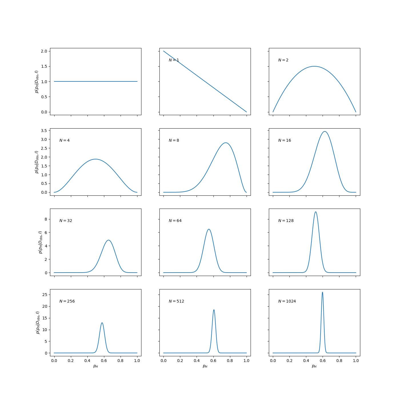
../../../_images/coinflipping_fig_1.png — Fig. 15.1 The evolution of the posterior pdf for the bias-weighting of a coin, as the number of data available increases. The figure on the top left-hand corner of each panel shows the number of data included in the analysis.#

The panel in the top left-hand corner shows the posterior pdf for \(p_H\) given no data, i.e., it is the same as the prior pdf of Eq. (15.11). It indicates that we have no more reason to believe that the coin is fair than we have to think that it is double-headed, double-tailed, or of any other intermediate bias-weighting.

The first flip is obviously tails. At this point we have no evidence that the coin has a side with heads, as indicated by the pdf going to zero as \(p_H \to 1\). The second flip is obviously heads and we have now excluded both extreme options \(p_H=0\) (double-tailed) and \(p_H=1\) (double-headed). We can note that the posterior at this point has the simple form \(p(p_H|D,I) = p_H(1-p_H)\) for \(0 \le p_H \le 1\).

The remainder of Fig. Fig. 15.1 shows how the posterior pdf evolves as the number of data analysed becomes larger and larger. We see that the position of the maximum moves around, but that the amount by which it does so decreases with the increasing number of observations. The width of the posterior pdf also becomes narrower with more data, indicating that we are becoming increasingly confident in our estimate of the bias-weighting. For the coin in this example, the best estimate of \(p_H\) eventually converges to 0.6, which, of course, was the value chosen to simulate the flips.

Take aways: Coin tossing#

The Bayesian posterior \(p(p_H | D, I)\) is proportional to the product of the prior and the likelihood (which is given by a binomial distribution in this case).
We can do this analysis sequentially (updating the prior after each toss and then adding new data; but don’t use the same data more than once!). Or we can analyze all data at once.
Why (and when) are these two approaches equivalent, and why should we not use the same data more than once?
Possible point estimates for the value of \(p_H\) could be the maximum (mode), mean, or median of this posterior pdf.
Bayesian p-precent degree-of-belief (DoB) intervals correspond to ranges in which we would give a p-percent odds of finding the true value for \(p_H\) based on the data and the information that we have.
The frequentist point estimate is \(p_H^* = \frac{H}{N}\). It actually corresponds to one of the point estimates from the Bayesian analysis for a specific prior? Which point estimate and which prior?