20. Bayesian Linear Regression#
“La théorie des probabilités n’est que le bon sens réduit au calcul”
(trans.) Probability theory is nothing but common sense reduced to calculation.
—Pierre Simon de Laplace
In this chapter we use Bayes’ theorem to infer a (posterior) probability density function for parameters of the linear model, conditional on \(\data\). This approach expands on the ordinary linear regression method outlined in Section 7. If you have not read that chapter yet, please do so now since we will build on this and also use some of the notation introduced there.
The advantages of doing Bayesian instead of ordinary (frequentist) linear regression are many. The Bayesian approach yields a probability distribution for the unknown parameters and for future model predictions. It also enables us to make all assumptions explicit whereas the frequentist approach puts nearly all emphasis on the collected data.
In the Bayesian approach to parameter estimation we start from Bayes’ theorem (18.3) which implies that we must make (prior) assumptions for the model parameters. In most realistic data analyses we will then have to resort to numerical evaluation (or sampling) of the posterior. However, certain combinations of likelihoods and priors facilitate analytical derivation of the posterior. In this chapter we will explore one such situation and also demonstrate how we can recover the results from an ordinary least squares approach with certain assumptions. A slightly more general approach involves so called conjugate priors. This class of probability distributions have clever functional relationships with corresponding likelihood distributions that facilitate analytical derivation.
20.1. Bayes’ theorem for the normal linear model#
Recall from Section 7 that we are relating data \(\data\) to the output of a linear model expressed in terms of its design matrix \(\dmat\) and its model parameters \(\pars\)
For the special case of one dependent, response variable (\(\output\)) and a single independent variable (\(\inputt\)) the data set (\(\data\)) and the residual vector (\(\residuals\)) are both \(N_d \times 1\) column vector with \(N_d\) the length of the data set. The design matrix (\(\dmat\)) has dimension \(N_d \times N_p\) and the parameter vector (\(\pars\)) is \(N_p \times 1\).
In linear regression using the ordinary least-squares method we made a leap of faith and decided that we were seeking a “best” model with an optimal set of parameters \(\pars^*\) that minimizes the Euclidean norm of the residual vector \(\residuals\). We then found that these were given by the normal equation (7.12) with solution (7.13)
Let us instead consider a statistical model for these residuals which describe the mismatch between our model and observations as in Eq. (18.1). Knowledge (and/or assumptions) concerning measurement uncertainties, or modeling errors, then allows to describe the residuals as a vector of random variables that are distributed according to a PDF
where we introduce the relation \(\sim\) to indicate how a (random) variable is distributed.
A very common assumption is that errors are normally distributed with zero mean. As before we let \(N_d\) denote the number of data points in the (column) vector \(\data\). Introducing the \(N_d \times N_d\) covariance matrix \(\covres\) for the errors we then have
Having such a statistical model for the errors makes it possible to derive an expression for the data likelihood \(\pdf{\data}{\pars,\covres,I}\) (see below). Using Bayes’ theorem (15.4) we can then “invert” this conditional probability distribution and write the parameter posterior
To evaluate this posterior we must have expressions for both factors in the numerator on the right-hand side: the likelihood \(\pdf{\data}{\pars,\covres,I}\) and the prior \(\pdf{\pars}{I}\). Note that the prior does not depend on the data and the error model. The denominator \(\pdf{\data}{I}\), sometimes known as the evidence, becomes irrelevant for the task of parameter estimation since it does not depend on \(\pars\). It is typically quite challenging, if not impossible, to evaluate the evidence for a multivariate inference problem unless in some very special cases. In this chapter we will only be dealing with analytically tractable problems and will therefore (in principle) be able to evaluate also the evidence.
Discuss
Why is it possible to perform parameter estimation without computing the evidence?
Can you think of why it is so challenging to compute the evidence?
20.2. The likelihood#
Assuming normally distributed residuals it turns out to be straightforward to express the data likelihood. In the following we will make the further assumption that errors are independent. This implies that the covariance matrix is diagonal and given by a vector \(\sigmas\),
and \(\sigmai^2\) is the variance for residual \(\epsilon_i\).
Let’s first consider a single data \(\data_i\) and the corresponding model prediction \(M_i = \left( \dmat \pars \right)_i\). We are interested in the likelihood for this single data point
We can follow the recipe in Chapter 19.3: Error propagation (II): Changing variables, since the relation between data and residual is a simple linear transformation \(\data_i = \modeloutput_i + \varepsilon_i\), and find
where we used that \(\epsilon_i \sim \mathcal{N}(0,\sigmai^2)\). Note that the parameter dependence sits in \(\modeloutput_i \equiv \modeloutput(\pars, \inputs_i)\).
Furthermore, since we assume that the residuals are independent we find that the total likelihood becomes a product of the individual ones
where we note that the diagonal form of \(\covres\) implies that \(\left| \covres \right|^{1/2} = \prod_{i=0}^{N_d-1} \sigmai\) and that the exponent becomes a sum of squared and weighted residual terms
In the special case that all residuals are both independent and identically distributed (i.i.d.) we have that all variances are the same, \(\sigmai^2 = \sigmares^2\), and the full covariance matrix is completely specified by a single parameter \(\sigmares^2\). For this special case, the likelihood becomes
Caution
For computational performance it is always better (if possible) to write sums, such as the one in the exponent of (20.9), in the form of vector-matrix operations rather than as for-loops. This particular sum should therefore be implemented as \((\data - \dmat \pars)^T (\data - \dmat \pars)\) to employ powerful optimization for vectorized operations in existing numerical libraries (such as numpy in python and gsl, mkl for C and other compiled programming languages).
Two views on the likelihood
Since observed data is generated stochastically, through an underlying “data-generating process”, it is appropriately described by a probabibility distribution. This is the “data likelihood” which describes the probability distribution for observed data given a specific data-generating process (as indicated by the information on the right-hand side of the conditional).
View 1: Assuming fixed values of \(\pars\); what are long-term frequencies of future data observations as described by the likelihood?
View 2: Focusing on the data \(\data_\mathrm{obs}\) that we have; how does the likelihood for this data set depend on the values of the model parameters?
This second view is the one that we will be adopting when allowing model parameters to be associated with probability distributions. The likelihood still describes the probability for observing a set of data, but we emphasize its parameter dependence by writing
This function is not a probability distribution for model parameters. The parameter posterior, left-hand side of Eq. (20.4), regains status as a probability density for \(\pars\) since the likelihood is multiplied with the prior \(\pdf{\pars}{I}\) and normalized by the evidence \(\pdf{\data}{I}\).
20.3. The prior#
Next we assign a prior probability \(\pdf{\pars}{I}\) for the model parameters. In order to facilitate analytical expressions we will explore two options: (i) a very broad, uniform prior, and (ii) a Gaussian prior. For simplicity, we consider both these priors to have zero mean and with all model parameters being i.i.d.
The uniform prior for the \(N_p\) parameters is then
with \(\Delta\para\) the width of the prior range in all parameter directions.
The Gaussian prior that we will also be exploring is
with \(\sigma_\para\) the standard deviation of the prior for all parameters.
20.4. The posterior#
Given the likelihood with i.i.d. errors (20.9) and the two alternative priors, (20.11) and (20.12), we will derive the corresponding two different expressions for the posterior (up to multiplicative normalization constants).
Rewriting the likelihood#
First, let us rewrite the likelihood in a way that is made possible by the fact that we are considering a linear model. Given the quadratic dependence on model parameters in the exponent one can show (by performing a Taylor expansion of the log likelihood around the mode) that the likelihood becomes proportional to the functional form of a multivariate normal distribution for the model parameters
Note that this expression still describes a probability distribution for the data. The data dependence sits in the amplitude of the mode, \(\pdf{\data}{\optpars,\sigmares^2,I}\), and its position, \(\optpars = \optpars(\data) = \left(\dmat^T\dmat\right)^{-1}\dmat^T\data\). The latter is the solution (7.13) of the normal equation. Furthermore, the statistical model for the errors (here with \(\covres = \mathrm{diag}(\sigmares^2)\)) enter in the covariance matrix,
which can be understood as the curvature (Hessian) of the negative log-likelihood.
Exercise 20.1 (Prove the Gaussian likelihood)
Prove Eq. (20.13).
Hints
Identify \(\optpars\) as the position of the mode of the likelihood by inspecting the negative log-likelihood \(L(\pars)\) and comparing with the derivation of the normal equation.
Taylor expand \(L(\pars)\) around \(\optpars\). For this you need to argue (or show) that the gradient vector \(\nabla_{\pars} L(\pars) = 0\) at \(\pars=\optpars\), and show that the Hessian \(\boldsymbol{H}\) (with elements \(H_{ij} = \frac{\partial^2 L}{\partial\para_i\partial\para_j}\)) is a constant matrix \(\boldsymbol{H} = \frac{\dmat^T\dmat}{\sigmares^2}\).
Compare with the Taylor expansion of a normal distribution \(\mathcal{N}\left( \pars \vert \optpars, \covpars \right)\).
Posterior with a uniform prior#
Let us first consider a uniform prior as expressed in Eq. (20.11). The prior can be considered very broad if its boundaries \(\pm \Delta\para/2\) are very far from the mode of the likelihood (20.13). “Distance” in this context is measured in terms of standard deviations. A “far distance”, therefore, implies that \(\pdf{\data}{\pars,\sigmares^2,I}\) is very close to zero. This implies that the posterior
simply becomes proportional to the data likelihood (with the prior just truncating the distribution at very large distances). Thus we find from Eq. (20.13)
if all \(\para_i \in [-\Delta\para/2, +\Delta\para/2]\) while it is zero elsewhere. The mode of this distribution is obviously the mean vector \(\optpars = \optpars(\data)\). We can therefore say that we have recovered the ordinary least-squares result. At this stage, however, the interpretation is that this parameter optimum corresponds to the maximum of the posterior PDF (20.16). Such an optimum is sometimes known as the maximum a posteriori, or MAP.
Discuss
In light of this result, what assumption(s) are implicit in linear regression while they are made explicit in Bayesian linear regression?
Posterior with a Gaussian prior#
Assigning instead a Gaussian prior for the model parameters, as expressed in Eq. (20.12), we find that the posterior is proportional to the product of two exponential functions
The second proportionality is a consequence of both exponents being quadratic in the model parameters, and therefore that the full expression looks like the product of two Gaussians. This product is proportional to another Gaussian distribution which has mean vector and (inverse) covariance matrix given by
where \(\boldsymbol{1}\) is the \(N_p \times N_p\) unit matrix. In effect, what has happend is that the prior normal distribution becomes updated to a posterior normal distribution via an inference process that involves a data likelihood. In this particular case, learning from data implies that the mode changes from \(\boldsymbol{0}\) to \(\tilde{\pars}\) and the covariance from a diagonal structure with \(\sigma_{\para}^2\) in all directions to the covariance matrix \(\tildecovpars\).
Discuss
What happens if the data is of high quality (i.e., the likelihood \(\mathcal{L}(\pars)\) is sharply peaked around \(\optpars\)), and what happens if it is of poor quality (providing a very broad likelihood distribution)?
Marginal posterior distributions#
Given a multivariate probability distribution we are often interested in lower dimension, marginal distributions. Consider for example \(\pars^T = [\pars_1^T, \pars_2^T\)], that is partitioned into respective dimensions \(D_1\) and \(D_2\). The marginal distribution corresponds to the integral
Transformation property of multivariate normal distributions
Let \(\mathbf{Y}\) be a multivariate normal-distributed random variable of length \(N_p\) with mean vector \(\boldsymbol{\mu}\) and covariance matrix \(\boldsymbol{\Sigma}\). We use the notation \(\psub{\mathbf{Y}}{\mathbf{y}} = \mathcal{N} (\mathbf{y} | \mathbf{\mu}, \mathbf{\Sigma})\) to emphasize which variable that is normally distributed.
Consider now a general \(N_p \times N_p\) matrix \(\boldsymbol{A}\) and \(N_p \times 1\) vector \(\boldsymbol{b}\). Then, the random variable \(\mathbf{Z} = \boldsymbol{A} \mathbf{Y} + \boldsymbol{b}\) is also multivariate normal-distributed with the PDF
For multivariate normal distributions we can employ a useful transformation property, shown in Eq. (20.19). Considering the posterior (20.17) we partition the parameters \(\pars^T = [\pars_1^T, \pars_2^T\)] and the mean vector and covariance matrix into \(\boldsymbol{\mu}^T = [\boldsymbol{\mu}_1^T,\boldsymbol{\mu}_2^T]\) and
We can obtain the marginal distribution for \(\pars_2\) by setting
which yields
20.5. The posterior predictive#
One can also derive the posterior predictive distribution (PPD), i.e., the probability distribution for predictions \(\widetilde{\boldsymbol{\mathcal{F}}}\) given the model \(M\) and a set of new inputs for the independent variable \(\boldsymbol{x}\). The new inputs give rise to a new design matrix \(\widetilde{\dmat}\).
We obtain the posterior predictive distribution by marginalizing over the uncertain model parameters that we just inferred from the given data \(\data\).
where both distributions in the integrand can be expressed as Gaussians. Alternatively, one can express the PPD as the set of model predictions with the model parameters distributed according to the posterior parameter PDF
This set of predictions can be obtained if we have access to a set of samples from the parameter posterior.
20.6. Bayesian linear regression: warmup#
To warm up, we consider the same situation as in Ordinary linear regression: warmup.
For the time being we assume to know enough about the data to consider a normal likelihood with i.i.d. errors. Let us first set the known residual variance to \(\sigmares^2 = 0.5^2\).
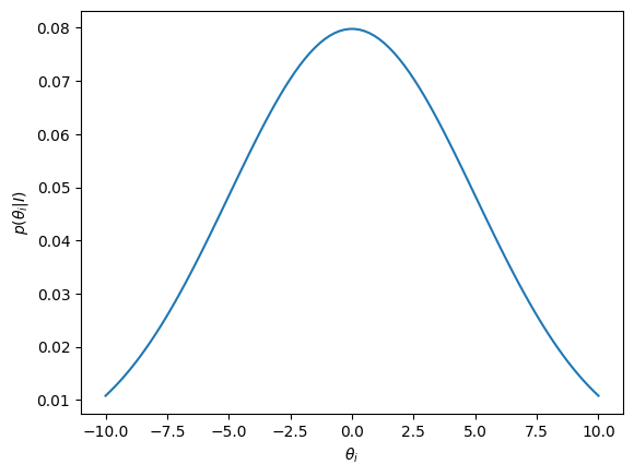
This time we also have prior knowledge that we would like to build into the inference. Here we use a normal prior for the parameters with \(\sigma_\para = 5.0\), which is to say that before looking at the data we believe \(\pars\) to be centered on zero with a variance of \(5^2\).
Let us plot this prior. The prior is the same for \(\theta_0\) and \(\theta_1\), so it is enough to plot one of them.
import numpy as np
import matplotlib.pyplot as plt
from scipy.stats import norm

def normal_distribution(mu,sigma2):
    return norm(loc=mu,scale=np.sqrt(sigma2))

thetai = np.linspace(-10,10,100)
prior = normal_distribution(0,5.0**2)

fig, ax = plt.subplots(1,1)
ax.plot(thetai,prior.pdf(thetai))
ax.set_ylabel(r'$p(\theta_i \vert I )$')
ax.set_xlabel(r'$\theta_i$');
It is straightforward to evaluate Eq. (20.18), which gives us
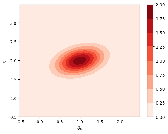
This should be compared with the parameter vector \((1,2)\) we recovered using ordinary linear regression. With Bayesian linear regression we start from an informative prior with both parameters centered on zero with a rather large variance.
Exercise 20.2 (Warm-up Bayesian linear regression)
Reproduce the posterior mean and covariance matrix from Eq. (20.23). You can use numpy methods to perform the linear algebra operations.
We can plot the posterior probability distribution for \(\pars\), i.e., by plotting the bi-variate \(\mathcal{N}-\)distribution with the parameter in Eq. (20.23).
from scipy.stats import multivariate_normal

mu = np.array([0.992,1.992])
Sigma = np.linalg.inv(4 * np.array([[2.01,-1.0],[-1.0,5.01]]))

posterior = multivariate_normal(mean=mu, cov=Sigma)

theta0, theta1 = np.mgrid[-0.5:2.5:.01, 0.5:3.5:.01]
theta_grid = np.dstack((theta0, theta1))

fig,ax = plt.subplots(1,1)
ax.set_xlabel(r'$\theta_0$')
ax.set_ylabel(r'$\theta_1$')
im = ax.contourf(theta0, theta1, posterior.pdf(theta_grid),cmap=plt.cm.Reds);
fig.colorbar(im);
Using Eq. (20.20) we can obtain, e.g., the \(\theta_1\) marginal density and compare with the prior
theta1 = np.linspace(-0.5,4.5,50)
mu1 = mu[1]
Sigma11_sq = Sigma[1,1]

posterior1 = normal_distribution(mu1,Sigma11_sq)

fig, ax = plt.subplots(1,1)
ax.plot(theta1,posterior1.pdf(theta1),'r-',\
label=r'$p(\theta_1 \vert \mathcal{D}, \sigma_\epsilon^2, I )$')
ax.plot(theta1,prior.pdf(theta1), 'b--',label=r'$p(\theta_1 \vert I )$')
ax.set_ylabel(r'$p(\theta_1 \vert \ldots )$')
ax.set_xlabel(r'$\theta_1$')
ax.legend(loc='best');
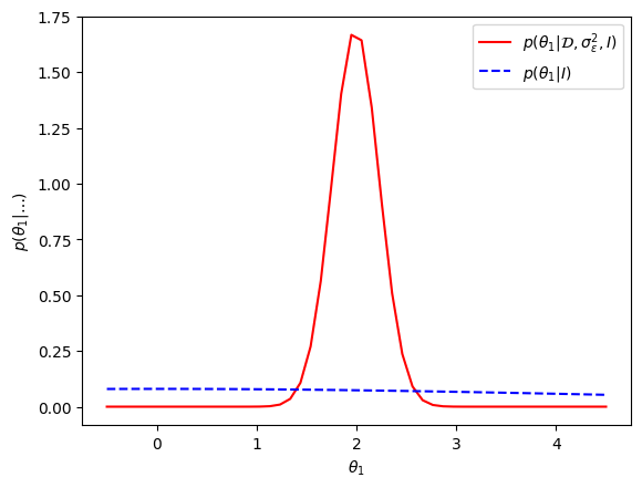
The key take-away with this numerical exercise is that Bayesian inference yields a probability distribution for the model parameters whose values we are uncertain about. With ordinary linear regression techniques you only obtain the parameter values that optimize some cost function, and not a probability distribution.
Exercise 20.3 (Warm-up Bayesian linear regression (data errors))
Explore the sensitivity to changes in the residual errors \(\sigmares\). Try to increase and reduce the error.
Exercise 20.4 (Warm-up Bayesian linear regression (prior sensitivity))
Explore the sensitivity to changes in the Gaussian prior width \(\sigma_\para\). Try to increase and reduce the width.
Exercise 20.5 (“In practice” Bayesian linear regression )
Perform Bayesian Linear Regression on the data that was generated in Ordinary linear regression in practice. Explore:
Dependence on the quality of the data (generate data with different \(\sigma_\epsilon\)) or the number of data.
Dependence on the polynomial function that was used to generate the data.
Dependence on the number of polynomial terms in the model.
Dependence on the parameter prior.
In all cases you should compare the Bayesian inference with the results from Ordinary Least Squares and with the true parameters that were used to generate the data.
20.7. Solutions#
Solution to Exercise 20.1 (Prove the Gaussian likelihood)
The likelihood can be written \(\pdf{\data}{\pars,I} = \exp\left[ -L(\pars) \right]\), where we include information on the error distribution (\(\sigmares\)) in the conditional \(I\). The negative log-likelihood, including the normalization factor, is
Comparing with Eq. (7.11) and the corresponding gradient vector (7.17) we find that
\[ \nabla_{\pars} L(\pars) = -\frac{\dmat^T\left( \data-\dmat\pars\right)}{\sigmares^2}, \]which is zero at \(\pars = \optpars = \left(\dmat^T\dmat\right)^{-1}\dmat^T\data\) corresponding to the solution of the normal equation.
We can Taylor expand \(L(\pars)\) around \(\pars=\optpars\) realizing that the linear (gradient) term is zero. Furthermore, the quadrating term depends on the second derivative (hessian) which is a constant matrix since \(L\) only depends quadratically on the parameters
Since higher derivatives therefore must be zero, the Taylor expansion actually terminates at second order
We introduce \(\covrespars^{-1} \equiv {\dmat^T\dmat} / {\sigmares^2}\) and use that \(\exp\left[ - L(\optpars) \right] = \pdf{\data}{\optpars,I}\). Therefore, evaluating \(\exp\left[ -L(\pars) \right]\) gives
\[ \pdf{\data}{\pars,I} = \pdf{\data}{\optpars,I} \exp\left[ -\frac{1}{2} (\pars-\optpars)^T \covrespars^{-1} (\pars-\optpars) \right], \]as we wanted to show.